Copyright © 2001-2006 DORSCH Consult
Copyright © 2007, 2014 Steffen Macke
Permission is granted to copy, distribute and/or modify this document under the terms of the GNU Free Documentation License, Version 1.2 or any later version published by the Free Software Foundation; with no Invariant Sections, no Front-Cover Texts, and no Back-Cover Texts. A copy of the license is available from the Free Software Foundation (http://www.gnu.org).
Table of Contents
- 1. DC Water Design Extension - General Information
- 2. DC Water Design Extension Reference
- Usage
- Analysis
- Frequently Asked Questions
- Why is there no graphical user interface to the DCWatDes.Bitcode.* functions?
- What is the Setup Dialog for?
- How do I recalculate the pipe length for all the pipes?
- I get strange errors when I try to create the EPANET model. What can I do?
- I made a mistake. Why is undo not working?
- How do I add rule-based controls?
- How do I add the initial status of a pump?
- I found a bug in the Extension. What should I do?
- How Can I Select All Rows where DC_ID is Longer than 13 Characters?
- How Can I Select All Rows where DC_ID Contains Spaces?
- Running "Make EPANET Model" Fails. What can I do?
- Development
- Copyright
- ArcView/EPANET Data Model
- 3. DC Water Design Extension Tutorials
- Index
List of Figures
List of Examples
This Manual describes the DC Water Design Extension Version 2.12.3.
This Document uses Terminology from ArcView and EPANET. Refer to the respective documentation for in-depth explanations.
![[Important]](images/important.png) | Important |
|---|---|
Be sure to check the DC Processing Extension and the DC Sewer Design Extension which are also freely available. These extensions provide additional functionality that is very helpful. E.g. the DC Sewer Design Extension can be used to draw water network profiles. |
The DC Water Design Extension is an Extension to ESRI's ArcView GIS software. Starting with Versions 2.00 the DC Water Design Extension integrates the EPANET 2.00 hydraulic modeling software with ArcView. It allows to store, edit and retrieve EPANET hydraulic models including all options in ArcView. Also it's possible to run the EPANET hydraulic analysis from ArcView and load the results into the GIS.
An Elevation calculation tutorial has been added to the extension (the section called “Elevation Assignment from Spot Heights”).
When writing EPANET INP files, the
Statusfield of aPipethat contains "closed" will be set to "closed".
Bytecode Calculator byte numbering starts with 1 now instead of 0.
"Extract Model" allows to select models that should be extracted as well as the folder to which the models should be extracted.
Robustness improvements for "Extract Model", "Split Model" and "Merge Model".
Fixed bug in "Split Model" and "Extract Model" that could lead to feature duplication when elements are moved from zone to zone in split models.
A Thiessen Polygon tutorial (the section called “Demand Calculation using Thiessen Polygons”) has been added to the documentation.
Experimental writing of OptiDesigner files (the section called “Write EPANET File”).
New function to select economic diameters based on the velocity result (the section called “Set Economic Diameter”).
Critical bug fixes for "Load Results for Step ...", "Extract Model", "Merge Model" and "Split Model". The bug could result in involuntary changes to the original data.
Bug fixes for
DCWatDes.Bitcode.or()andDCWatDes.Bitcode.xor()functions.Improved "Bytecode Calculator" functionality (the section called “Bytecode Calculator”).
"Write Epanet File" collapses setting entries of valves to "closed" if they contain "closed".
"Extract Model" allows now to create one view per model (the section called “Extract Model”) and will extract demand junctions to a separate file if a field
HasDemandis found in the junction table..New "Enforce Data Model" option that allows to relax data model checks when editing networks (E.g. sewer or street networks). See the section called “Setup”.
"Select Connected Pipes" looks for "closed" as a substring rather than a closed string (If "Closed Valve" is selected).
Bitcodes became byte codes (strings) and can distinguish up to 255 zones.
New "Split Model", "Merge Model" and "Extract Model" functions in the Project GUI (the section called “Split Model”, the section called “Merge Model”, the section called “Extract Model”).
INP file import is handling virtual lines now. Function robustness has been improved and error messages are displayed in ArcView.
More robust "Create Missing Junctions" function.
Updated documentation
New installer interface.
Bug fixes for patterns, help file integration, result import.
Switched Documentation to DocBook. Documentation is accessible from DC Water Design Extension Menu now.
Fixed pattern export
The extension doesn't use the power_kw field of the pump table any more.
Bug fix for result import.
Better handling of curves and patterns.
Improved "Check Epanet model" functionality.
Basic skeletonization function.
Bug fixes for the "Create Missing Junctions" function.
Russian localizations (Thanks to Tom Chidley).
More Arabic localizations (Thanks to Maher Karim).
Bug fixes for emitterexponent and demandmultiplier export to EPANET INP files.
Added emitter coefficient as to the junction class.
Updated documentation.
Completely new and much faster EPANET INP import based on the EPANET toolkit and shapelib. Import function still incomplete: Attributes are omitted.
French and Arabic localizations.
Bug fixes for one-node themes, snapping radius, pipe splitting, popup menus and exporting.
Fixed several problems when the view contained raster themes.
EPANET INP import: Fixed junction import, improved performance. Import function still incomplete.
Customizable timeout and other improvements for external command calls (Thanks to Melissa Henderson of Lockwood, Andrews & Newnam, Inc.).
Check EPANET model checks now for pipes that are shorter than the snapping radius.
Import of EPANET binary result files.
Preliminary support for importing EPANET INP files: Importing pipes and junctions.
Added function to automatically add the theme fields required by the data model.
EPANET result import works now without MySQL.
Check EPANET Model provides more checks now and is much faster.
"Create Missing Junctions": Add additional junctions to make sure that the network topology is sane.
Updated Documentation.
Checking for spaces in path names which are not allowed.
Customizable backdrop map resolution.
Support for patterns.
More checks while writing EPANET files.
Various bugfixes (see
ChangeLogfor the details).
Updated Documentation.
Support for Backdrop Maps (Thanks to Roland Salgado, the section called “Write EPANET File”).
Create Zones From SOV Controls (the section called “Create Zones from Controls”).
Bugfix for coordinate systems using decimal feet (Bug reported by Arnold Strasser).
This section introduces some concepts which are fundamental in order to understand how the extension works.
Network Traces can be useful to solve problems related to the network geometry. For example, it's possible to check the connectivity of the network features in a model. Through specifying network features at which the trace should stop, it's possible to isolate supply zones.
In the EPANET hydraulic model, pumps and valves are represented as lines. From the hydraulic modeling point of view this makes sense, as the orientation of the valves and pumps is important information. In GIS data, pumps and valves are typically represented as points, as they are also symbolized with point symbols. Point data is lacking the orientation information. Because of the pipe-node duality pipes and valves will be referred to as virtual lines in this section.
The pipe-node duality complicates the creation of hydraulic models from the GIS data. It is possible to overcome the problem with one of the following solutions:
Storage of orientation information for each virtual line in the GIS
Take over the orientation of connected pipes
The second possibility has some advantages, as it does not require additional data storage - it was applied in the described application. However, it imposes some restraints on the data. The concept to model virtual lines as points in the GIS can be summarized as follows:
Each virtual line needs to have exactly two pipes connected
Both connected pipes must be oriented in the same way: One pipe has to start at the virtual line and the other pipe has to end at the virtual line
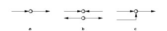
Figure 1.1, “Virtual Line Validity” shows examples of different
pipe orientations
at a virtual line. The case a shows a pump with two
pipes connected that are oriented in the same way. This
allows the creation of the hydraulic model and is
therefore considered valid. Case b shows pumps with
pipes connected that are not oriented in the same way.
This is invalid as is does not allow the creation of
the hydraulic model. Case c is invalid because the pump
has more than 3 pipes connected to it. Note that the
orientation information of the pump symbol is not
necessarily contained in the GIS data.
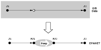
Figure 1.2, “Virtual Line Creation”
depicts the conversion process of virtual
lines:
Number and orientation of the pipes connected to the virtual line are checked for validity
The virtual node is replaced with a junction (PJ1).
An additional junction is added (PJ2).
The pipe from the virtual line to the next node starts at the additional junction. (PJ2 -> J2).
The pump or valve is created. It connects the two new Junctions (PJ1 -> PJ2).
The DC Water Design Extension follows this conversion process when it is creating EPANET models. Additional considerations used in the process are:
The length of the virtual line is one metre. Figure 1.2, “Virtual Line Creation”
If the pipe starting at the virtual line is shorter than one metre, the virtual line length is set to half of the pipe length.
Virtual Lines provide a concept to convert GIS point data (pumps or valves) into the lines used by the hydraulic analysis software. The conversion is done automatically when the GIS data is exported to the hydraulic model. Virtual Lines require exactly two pipes connected to each pump or valve. In Addition, the two pipes have to have the same digitizing direction (which will be the flow direction in the hydraulic model).
Byte codes make it possible to store fields of yes-no information in 'normal' text. Every byte in the number having the value "1" is considered set, every byte of value "0" is not set. Thus making it possible to code several independent pieces of information in one ArcView string.
As ArcView shapefiles allow to store strings of up to 255 characters length, it is possible to store up to 255 pieces of information.
The following example shows how this concept allows storing the network information in one seamless data set and utilizing the same network features in different hydraulic models:
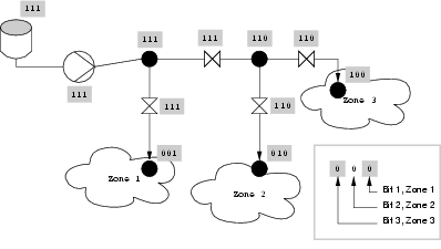
In Figure 1.3, “Byte-coding Supply Zones” the nodes of three hydraulic models are byte-coded for storage in the GIS. Each zone has its own byte in the byte code, indicating if the node is used in the model or not.
Byte codes are stored as strings in GIS data. They provide a powerful method to store hydraulic models in GIS data. The underlying principle is very simple:
The models are numbered
Each byte represents one supply zone
If the byte is set ("1") than the network feature is used in the respective model. Otherwise ("0"), the feature is not used in the model.
The different values are assembled by the following functions:
DCWatDes.Bitcode.and DCWatDes.Bitcode.or DCWatDes.Bitcode.xor See the section called “API Documentation” for details regarding these functions.
![[Note]](images/note.png) | Note |
|---|---|
Note that the byte numbering starts at 1. You should use a temporary field in order to perform the addition of two byte codes correctly. |
| Note |
|---|---|
Note that you should use a different concept if you want to split up your model for editing purposes. The byte code concept models a one to many relationship, but for editing purposes, a one to one relationship should be used. This makes the automatic assembly of the model after editing easier. |
Description of the DC Water Design Extension Installation.
The DC Water Design Extension can be obtained from the website http://dcwaterdesign.sourceforge.net.
The sourceforge site offers a multitude of services related to the DC Water Design Extension, including:
Downloads
Documentation
Sources
Bug Tracker
Mailing List
Sample Data
The following software packages are required in order to use the DC Water Design extension:
ArcView 3.1 or higher (3.2, 3.3), but not ArcView 8.x or 9.x
Windows 95, 98, ME, NT, 2000 or XP in order to export EPANET files
EPANET 2.0 or higher is needed in order to run a hydraulic analysis
An (ANSI SQL compliant) ODBC connection can improve the performance when importing hydraulic analysis results
| Note |
|---|---|
Note that the commandline tools described in the section called “Commandline Tools” do not rely on ArcView or the Windows operating system. They are platform independent, however you may have to compile them for your platform. |
To install the DC Water Design Extension, you've got to
run the installer executable. After accepting the
license (s. the section called “DC Water Design Extension”), you'll be
prompted to select the
installation path. The installation path should be the
path to ArcView's EXT32 folder. Usually this should be
the default path (c:\ESRI\av_gis30\arcview\EXT32). It
might differ for custom ArcView installations. The only
thing left to do now is to select which components of
the extension should be installed. In general, you
should install all the components of the extension.
| Note |
|---|---|
If you want to use e.g. a newer version of the XSLT parser and you've installed that version already, you might decide not to install the XSLT parser that comes with the extension. Don't do this unless you know what you're doing! |
Load the Extension.
Open a View.
Add Themes to the View. The Themes should describe your water supply network. Junctions, pipes and reservoirs would comprise a simple network. The attributes of the themes must adhere to the ArcView/EPANET Data Model (see the section called “ArcView/EPANET Data Model”). You can use ArcView field aliases to map the fields correctly.
Click on the EPANET Themes button. Select the appropriate Themes.
If your fieldnames don't match the ones of the data model, choose "Create Missing Fields" from the DC Water Design menu.
If required, use the ArcView table calculator to populate the fields. Leaving fields empty is fine in most cases.
Choose "Make EPANET Model" from the DC Water Design menu.
If the last step didn't yield any errors, you can create an EPANET input file now. Choose "Write EPANET File" from the DC Water Design menu. Choose filename and location. In case of errors, running "Check EPANET Model" might help you to track down the most common error.
Fire up EPANET and open the created file (*.inp).
How to use the DC Water Design Extension.
Start ArcView
Open the Extensions Dialog ( → )
Select the DC Water Design Extension (Put a checkmark in the box on the left side).
After the Extension is loaded, the Setup Dialog informs you about several settings. You shouldn't change them without knowing what you're doing.
The DC Water Design Extension extends the Project GUI by adding a new Menu, called DC Water Design Extension. The Menu contains the following choices:
Shows the Setup Dialog.
The Setup Dialog includes an option to choose the language of the Extension. Currently supported are the following localizations:
Arabic
English
German
Russian
| Note |
|---|---|
Note that the Localization is not completed yet. It is therefore recommended that you set the language to English. |
The snapping radius used for network traces and model building is also customizable in this dialog. Usually the default setting should be kept.
The backdrop resolution specifies the resolution of the backdrop map if you write your EPANET files with backdrop maps. Set to a higher resolution if required.
The command timeout specifies the time in seconds for which the extension will wait when creating epanet files or running epanet calculations. If the EPANET run doesn't finish in time, there'll be an error message.
Deselecting the Enforce Data Model checkbox allows to relax checks on fields required for EPANET.
![[Tip]](images/tip.png) | Tip |
|---|---|
Deselect the Enforce Data Model checkbox when editing street or sewer networks. |
Displays the EPANET Tables Dialog.
The Tables in the dialog are used to to store non-spatial EPANET data with ArcView. Typical examples of such data are pump curves or hydraulic analysis options. Before you can choose a table to use with the DC Water Design Extension, it has to be loaded into ArcView. Refer to the ArcView documentation for information on how to load tables into ArcView.
Opens the Result Tables Dialog.
The Result Tables are used to store the results of a hydraulic analysis. There are two tables, one for node results and one for link results. For performance reasons it is recommended that you use a RDBMS such as mySQL for storing the data.
To allow result file loading without having an RDBMS installed, the dialog provides the opportunity to switch to an result loader that relies on ArcView only.
Allows to split a model into different ones.
The values of the Zone field will
be used to determine to which model a network element belongs
The sub-models will be stored in subfolders named like the zones.
the section called “Merge Model” can be used to re-assemble the model automatically.
![[Caution]](images/caution.png) | Caution |
|---|---|
The |
Merge a model that was split by the section called “Split Model”.
Because "Merge Model" is using the zone names from the main pipes theme, it is not possible to add new zones by simply adding a new folder. New zones have to be introduced in the main file first.
| Caution |
|---|---|
The |
Extract separate models from the current one based on
the ByteCode content.
Splits the currently registered themes into several parts.
The parts are stored in the model folder
and numbered according to byte code that is set. For example,
all network elements with the first byte set (E.g. "1000")
are stored in the folder model/1.
The user is asked whether a new view should be created for each model. The views will be named "Model 1", "Model 2"...
If the junction theme has a HasDemand
field and its filename contains "junction", additional
demandjunction.shp files will be written
to the folder. They contain all the records for the particular model
where HasDemand is "1".
The definition query for all themes of the model will be removed by this operation.
See the section called “Byte Codes” for detailed information about byte codes.
Unlike the section called “Split Model” and the section called “Merge Model” this function support one-to-many relationships (One pipe can be part if different models).
Displays information about the DC Water Design Extension License. See section the section called “DC Water Design Extension” for the license details.
The DC Water Design Extension extends the ArcView View GUI with the following elements:
A new Menu called "DC Water Design"
Buttons
Tools
Three pop-up menus
The pop-up menus are available through clicking the right mouse button over a network feature.
The additional functionality is explained below.
Exports the hydraulic model to an EPANET input file.
The model has to be complete, running "Make EPANET Model" and "Check EPANET Model" is advisable especially for the novice user before exporting the EPANET input file.
The typical process that follows "Write EPANET File" is outlined in Figure 2.1, “Write EPANET File”. Note how this differs from the process in Figure 2.2, “Run EPANET Calculation”.
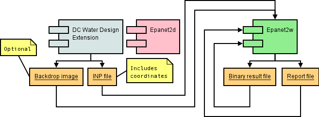
Optionally, a Backdrop Map is exported together with the EPANET model. This requires additional themes in the View e.g. pressure zones or a street layer. The resolution of the backdrop map can be specified in the setup dialog (see the section called “Project Menus”). A backdrop will only be written, if the view contains visible themes in addition to the EPANET themes.
If the Status field of a Pipe or the Setting field of
a Valve contains "closed", it will be
set to "closed".
| Note |
|---|---|
The resulting EPANET input file has the extension *.inp. The *.xml-file is just an intermediate format (temporary file). |
| Note |
|---|---|
The function is writing experimental OptiDesigner files
( |
Exports the hydraulic model to an EPANET input file, runs the analysis and loads the results into ArcView.
The typical "Run EPANET Calculation process" is outlined in Figure 2.2, “Run EPANET Calculation”. Note how this differs from the process in Figure 2.1, “Write EPANET File”.
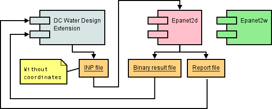
The model has to be complete, running "Make EPANET Model" and "Check EPANET Model" is advisable especially for the novice user before exporting the EPANET input file.
After the analysis has been completed, the report created by EPANET is displayed in a window and the user is prompted to select a time step for which the results will be loaded.
Loads binary results of an EPANET calculation into ArcView.
The binary results need to result of from an analysis of the EPANET model currently loaded into ArcView.
The user will be prompted to select a time step for which the results will be loaded.
Imports an EPANET model from an EPANET INP file.
The EPANET INP format is an ASCII format (it can be easily edited by any text editor) that is documented in the EPANET toolkit. The windows version of EPANET can export models to this format. To export an INP file from EPANET, choose → → ) from the menu.
After selecting → from the menu, you have to do the following:
Select the location for the new
Junction shapefile to be created. |
Select the location for the new
Pipe shapefile to be created. |
Select the location for the new
Pump shapefile to be created. |
Select the location for the new
Reservoir shapefile to be created. |
Select the location for the new
Tank shapefile to be created. |
Select the location for the new
Valve shapefile to be created. |
| Select the EPANET INP file to be imported. |
If there are errors, they will be reported in a separate window.
| Caution |
|---|---|
Currently the function will not import the full EPANET model. Be sure to check whether the imported results fit your needs. |
The function uses the inp2shp command. (the section called “inp2shp”).
Performs a number of checks on the hydraulic model.
The checks include the following:
Check for NULL shapes
Check for pipes shorter than the snapping radius
Check for duplicate IDs
Check for IDs that are too long
Loads the results of an EPANET hydraulic analysis to ArcView.
The hydraulic analysis has to be run from ArcView in order to to enable this feature. The user is prompted to select the time step for which the results should be loaded.
Creates the line-node structure required by EPANET.
This function fills the fields node1 and node2 in the links table with the dc_ids of the connected nodes. The fields will be overwritten by this function, therefore the user has to confirm the action before the script run.
After completion, a report gives a overview of the created model. Model creation errors are also reported. If there were errors, the features in question are selected after the run.
In case there are reports about inconsistent flow direction at pumps or valves, you can use the "Flip Polylines" tool to correct the errors (the section called “Flip Polylines”).
| Tip |
|---|---|
Increase the snapping radius if necesary (the section called “Setup”. |
Opens the EPANET Themes Dialog.
Use the Dialog to select the themes you want to use in your hydraulic model. The line and node theme are required, other themes are optional and can be switched off with the check boxes on the right side.
| Important |
|---|---|
Most of the extension functions require that the EPANET Themes are properly set up in this dialog. |
Setting up the themes should be the first step when using the extension. The settings are also used to determine which themes should be edited.
Displays the EPANET Tables Dialog.
The Tables in the dialog are used to to store non-spatial EPANET data with ArcView. Typical examples of such data are pump curves or hydraulic analysis options. Before you can choose a table to use with the DC Water Design Extension, it has to be loaded into ArcView. Refer to the ArcView documentation for information on how to load tables into ArcView.
Allows to set valve states according to EPANET Controls.
If a controls table is registered with the Extension (see the section called “EPANET Tables”), the user is offered to select the controls he would like to apply. All chosen controls are applied. This is very useful in combination with Network Traces as the extension allows to stop traces at closed valves.
Creates a straight pipe between tanks and junctions which share an id.
This function requires some preparatory work: Each tank of the tanks theme needs to know to which junction he should be connected. This is expressed with a field in the tanks attribute table that contains the dc_id of the junction the tank should connect to. Such fields can be established e.g. by using the spatial join function of the Geoprocessing Wizard.
| Note |
|---|---|
Note that this functionality has been included mainly for the purpose of modeling intermittent supply with household storage tanks. |
It might be taken out or completely rewritten in future versions of the DC Water Design Extension.
Calculates a coded text that shows when a node is supplied with water.
This might only be used after successfully running an EPANET hydraulic analysis from ArcView. The function will query the the nodes results table for pressures above zero. Each pressure above zero will yield a "1" in the supply string, a pressure below or equal zero will yield a "0" in the supply string. For each node, the supply strings are written to a user-selectable text field. The field has to been long enough to contain as many characters as there are time steps in the EPANET results.
| Note |
|---|---|
Note that this functionality has been included mainly for the purpose of modeling intermittent supply with household storage tanks. |
It might be taken out or completely rewritten in future versions of the DC Water Design Extension.
This function calculates the length of the pipes connected to a junction.
A user selectable number field in the junctions attribute table is filled with the length of the pipes connected to each junction. In order not to double the overall pipe length, each pipe length is divided by two. Thus every part of a pipe is assigned to the nearest node.
Creates new themes with features which have the same bit set in a bit code.
The function works with all active themes in the view. First, the user is prompted to select the bit which has to be set for the clipped themes. Then the field containing the bit code has to be chosen. (The script assumes that the bit code field names are the same throughout all the active themes.) The user can select the filename and location for each clipped theme. He can also choose whether the new themes should be added to the view.
Creates a sequence (string) of 0 and 1 for describing if the pipe is connected to a reservoir at over a sequence of hours.
A user selectable text field in the pipe attribute table is filled with a string containing 0's and 1's. The n-th character is a 0 if the pipe is not connected to a reservoir in the n-th hour or 1 if the pipe is connected.
A string "00111" means that the pipe was supplied from the second to the fifth hour.
Such information can be used to automatically determine zones for networks with intermittent supply. Zones are disconnected by the shut off valves. The shut off valves are controlled by the controls table. The supported control syntax is:
LINK link_id status AT TIME hours_since_simulation_start
The number of traces - which is equal to the number of hours from simulation start - can be chosen by the user. The function requires the Epanet model to be set up correctly (Including valves and controls).
Currently the function only supports networks that contain only shut off valves.
Creates fields required by the data model if they are missing in the EPANET themes.
This allows to quickly create data sets that conform with the EPANET data model.
Tools that are added to the View GUI.
This tool allows to flip the digitizing direction of lines.
The theme containing the lines to be flipped has to be set up as the pipe theme in the EPANET themes dialog. Simple clicking on the line will switch the digitizing direction.
| Tip |
|---|---|
ArcView's symbology can be used to display the digitizing direction with arrowheads. |
A tool to move network nodes including rubber-banding.
With this tool it's possible to move network nodes (junctions, tanks, reservoirs, pumps, valves) along with the connected pipes. The network stays intact and fully connected (rubber-banding).
The respective themes have to be registered with the extension in the EPANET themes dialog.
Tool that allows to split a pipe into two pipes. Adds a new junction at the split point.
The two new pipes inherit the attributes from the original pipe. However, the length gets recalculated based on the shapes.
Pipe and junction themes have to be chosen in the EPANET themes dialog.
Allows to re-shape pipes.
Vertices determine the route of a pipe. The tool makes it possible to move all the vertices of a pipe. Additional, it's possible to add vertices to the pipe. Unlike the ArcView tool "Vertex Edit", "Edit Pipe Vertices" ensures network connectivity - it is impossible to disconnect a pipe from a node with this tool.
The pipe theme has to be set up in the EPANET themes dialog in order to use this tool.
| Important |
|---|---|
Note that the pipe length is not recalculated. |
Recalculate the pipe length manually in the pipe theme attribute table. See the Questions and Answers section of this manual if you have problems calculating the pipe length.
Tool to convert nodes from one class to another.
The Change Node Class tool allows to convert e.g. a junction into pump. Attributes shared between the two classes are copied. After selecting an existing node, the user is prompted to select the class to which the node should be moved. The old node is deleted.
Obviously, the respective themes have to be registered with the extension in the EPANET themes dialog.
A tool to delete network features.
Allows one-click deletion of network features. The user is prompted to confirm the deletion. Remember that there's no undo support with the DC Water Design Extension.
The themes containing features that should be deleted have to be selected in the EPANET Themes dialog.
The Digitize Junction tool is used to digitize junctions.
The junctions are added to the junction theme selected in the EPANET themes dialog.
The Digitize Pipe tool is used to digitize pipes.
The pipes are added to the pipe theme selected in the EPANET themes dialog. In order to maintain the network integrity, the tool automatically adds junctions at the pipe end if the pipe end doesn't snap onto an existing node.
The Digitize Tank tool is used to digitize tanks.
The tanks are added to the tank theme selected in the EPANET themes dialog.
The Digitize Valve tool is used to digitize valves.
The valves are added to the valve theme selected in the EPANET themes dialog. The tool is disabled if the valve theme is not enabled in the EPANET themes dialog.
The context menu items described in this section are available if the right mouse button is pressed over a theme that has been registered with the DC Water Design Extension (See the section called “EPANET Themes”).
Pop-up menu item that allows to show the attributes of a pipe.
Right-clicking on a pipe and selecting this menu item opens the pipe attribute table, selects and promotes the pipe.
The appropriate pipe theme has to be selected in the EPANET themes dialog.
Pop-up menu item allowing to edit the attributes of a pipe.
Right-clicking on a pipe and selecting this menu item opens the pipe attribute table, makes it editable, selects and promotes the pipe record. After that, the attributes of the pipe can be edited. Keep in mind that there's no undo.
Pop-up menu item that allows to trace the pipes connected to the selected pipe.
Right-clicking on a pipe and selecting this menu item opens a dialog that offers node types at which the trace should stop. Multiple types can be selected. During the trace, the status bar informs what percentage of the network has been covered by the trace so far. Note that the progress bar won't make it to 100% unless the network is fully connected and no stopper has been selected. The connected pipes up to all stop points are returned as the selection.
| Tip |
|---|---|
The option "Closed Valves" will stop if
a feature in the valve theme contains the text "closed" in
the field |
Interactively traces connected pipes.
See the section called “Select Connected Pipes” for more information on network traces.
Select the pipe diameter from a list. The economic diameter will be selected by default based on the flow rate result.
Example 2.1. Economic Diameter Selection
The field result_flow of the pipe table contains a value of 15 l/s. In this case a DN 150 pipe will be suggested. The resulting velocity will be 0.85 m/s.
| Important |
|---|---|
This function only works when "LPS" units are used (Field Units of the EPANET options table). |
Pop-up menu item that shows the attributes of a node.
Right-clicking on a node and selecting this menu item opens the node attribute table, selects and promotes the pipe.
The appropriate node theme has to be selected in the EPANET themes dialog.
Pop-up menu item that allows to edit the attributes of a node.
Right-clicking on a node and selecting this menu item opens the node attribute table, makes it editable, selects and promotes the node record. After that the attributes of the node can be edited. Keep in mind that there's no undo.
Table buttons that are added by the extension.
The Bytecode Calculator is accessible from the button bar of the table GUI. It is disabled unless the table is editable and a numerical field is selected.
Upon clicking on the Bytecode Calculator button, the user is prompted to select the bits he wants to set.
After choosing OK, the bit code will be calculated and written to all the selected records.
If no records are selected the bit code is written to all the records in the table.
The field used to store the byte codes should have no decimal places.
See the section called “Byte Codes” for details regarding byte codes.
Several commandline tools that are available together with the DC Water Design Extension.
If you do not know what a commandline tool is, you may want to skip this section as the DC Water Design Extension provides
Note that these tools don't rely on ArcView and may be used independent of the DC Water Design Extension.
Converts EPANET INP files to a group of shapefiles that conform to the EPANET/ArcView data model.
Used by the EPANET INP import function (the section called “Import EPANET Inp File”).
The command is used as follows:
inp2shpmodel.inp
model.txt
j.shp
p.shp
pu.shp
r.shp
t.shp

| The inp2shp program. |
| The INP file to be imported. Replace with the path to your INP file. |
| A report file to be generated by the EPANET engine. The file might contain additional error message that can help to track down problems. Existing file will be overwritten! |
| The junction shapefile to be generated or overwritten. Replace with the path to save the junction shapefile. Existing files will be overwritten! |
| The pipe shapefile to be generated or overwritten. Replace with the path to save the pipe shapefile. Existing files will be overwritten! |
| The pump shapefile to be generated or overwritten. Replace with the path to save the pump shapefile. Existing files will be overwritten! |
| The reservoir shapefile to be generated or overwritten. Replace with the path to save the reservoir shapefile. Existing files will be overwritten! |
| The tank shapefile to be generated or overwritten. Replace with the path to save the tank shapefile. Existing files will be overwritten! |
Shapefiles will only be generated for those network elements that are included in the INP file.
Virtual lines are processed as required (See the section called “Virtual Lines”).
| Important |
|---|---|
Make sure that inp2shp.exe and
the patched |
Convert binary EPANET result files to comma separated ASCII files.
Used by several functions (the section called “Run EPANET Calculation”, the section called “Import Binary Result File”, the section called “Load Results for Step ...”)
How the results can be analyzed.
How to import the results to R:
node <- read.csv("c:\\temp\\node.txt",header=TRUE)The provided AVENUE functions are more flexible this way. Bit codes can be useful for quite a number of operations. Try using the functions with the field calculator and the query. Examples are given in the section called “API Documentation”.
The Extension depends on several software packages. The Setup Dialog allows you to use other versions of these software packages than the ones supplied with the Extension itself.
Open the attribute table of the pipe theme.
Make sure that the pipe theme is editable.
Make sure that no records are selected.
Click on the heading for the length field.
Click on the field calculator button.
Enter the following line into the value field:
[Shape].returnLength
Click OK.
Try the following:
Try "Check EPANET model". This should help you to resolve duplicate IDs.
Have a close look at the erroneous features: Often accidentally duplicates features cause trouble. Tools like JUMP can help to identify duplicate features
| Important |
|---|---|
Undo support had to be taken out for the sake of editing multiple themes at the same time. Make frequent backups. |
You've been warned.
If you have a text file for simple controls, add lines like the following to it:
[RULES]

      RULE 1 IF TANK LEVEL 1 ABOVE 19.1

THEN PUMP 355 STATUS IS CLOSEDJust add it to the properties field of the pump like in the following example:
HEAD Curve1 SPEED 1.2
Please send your bug reports to
<dcwaterdesign-info@lists.sourceforge.net> or
use the bug tracker on the website.
Closely analyse the selected records.
Try to increase the snapping radius (the section called “Setup”).
This section contains information that is relevant to developers. Most probably you only want to read this if you are a programmer.
This section documents extension scripts that could be used from the field calculator or in queries. In Addition, the script responsible for the extension dictionaries is documented. In general, the API documentation should only be of concern for programmers.
DCWatDes.Bitcode.or performs a bytewise or operation on string numbers.
string DCWatDes.Bitcode.or(string a, string b)
a byte-coded string
b byte-coded string
Returns: the result of the bytewise a or b as a string
The following AVENUE code can be used in the field calculator to perform of a bytewise or-operation on the fields a and b:
av.run("DCWatDes.Bitcode.or", {[a], [b]})
DCWatDes.Bitcode.xor performs a bytewise xor operation on string numbers.
string DCWatDes.Bitcode.xor(string a, string b)
a byte-coded string
b byte-coded string
Returns: the result of the bytewise a xor b as a string
The following AVENUE code can be used in the field calculator to perform of a bytewise or-operation on the fields a and b:
av.run("DCWatDes.Bitcode.xor", {"111", "101"})
The result of the example above will be "111".
DCWatDes.Bitcode.and performs a bytewise and operation on string numbers
string DCWatDes.Bitcode.and(string a, string b)
a bit-coded string
b bit-coded string
Returns: the result of the bytewise a and b as a string
The following AVENUE code can be used in the field calculator to perform of a bytewise and-operation on the fields a and b:
av.run("DCWatDes.Bitcode.and", {[a], [b]})
DCWatDes.Bitcode.isSetAsNumber returns whether the n-th byte of a string is set or not
integer DCWatDes.Bitcode.isSetAsNumber(string a, integer n)
a byte-coded string
n number of the byte to check
Returns: an integer of value 1 in case the n-th byte is set, 0 otherwise
The following AVENUE query can be used to select all the records which have set the 4th bit in the example field (usable with the query tools of view and table GUI):
   av.run("DCWatDes.Bitcode.isSetAsNumber",{"0001", 3})
   = 1
The expression will return true
Note that the bit numbering starts at 0. "= 1" is used to convert the numbers 0 and 1 to the boolean values to true or false, respective.
| Tip |
|---|---|
Note that you can also use the "0001".middle(3,1) = "1"
|
Creates the Localization dictionaries of the Extension
In order to add another Dictionary, you'll first have to create one:
dicNew = Dictionary.make(100)
Then you can start adding dictionary entries:
dicNew.add("English Term", "New translated term")Look at the German dictionary for the terms that have to be translated. After you've added all the terms to the new Dictionary, you have to add the Dictionary to the Dictionary of Dictionaries:
_dcwDicDictionaries.add("de", dicNew)
Where "de" is describes the locale (In this case "de" for Germany).
Updates the valves status field, reflecting the status at a given time.
All valves are closed before applying the controls.
Expects the timestep as a number as the argument (Hours since simulation start).
Returns nothing.
Requires valves theme and controls table registered with the extension.
Works only for SOV valves. The supported controls syntax is:
LINK link_id status AT TIME hours_since_simulation_start
Procedures in the development process.
Steps that should be followed in the release process.
Update the version number in
dcwatdes2.apr,build.xml,doc/en/dcwaterdesign.xml,installer/dc_water_design_extension.nsi.Build the documentation using ant and
doc/build.xml.Build the installer using NSIS and
installer/dc_water_design_extension.nsi.Test the installer.
Build the source zip file using ant and
build.xml.Upload the files to ftp://upload.sourceforge.net/incoming/
Create the release on Sourceforge.
Create a Sourceforge news item
Announce the release on the EPANET, DC Water Design mailing lists.
Copyright information for the various components of the DC Water Design Extension.
DC Water Design Extension. This ArcView Extension integrates EPANET with ArcView.
Copyright (C) 1998-2005 DORSCH Consult
This library is free software; you can redistribute it and/or modify it under the terms of the GNU Lesser General Public License as published by the Free Software Foundation; either version 2.1 of the License, or (at your option) any later version.
This library is distributed in the hope that it will be useful, but WITHOUT ANY WARRANTY; without even the implied warranty of MERCHANTABILITY or FITNESS FOR A PARTICULAR PURPOSE. See the GNU Lesser General Public License for more details.
You should have received a copy of the GNU Lesser General Public License along with this library; if not, write to the Free Software Foundation, Inc., 59 Temple Place, Suite 330, Boston, MA 02111-1307 USA
testXSLT (Xalan C++) Copyright (C) 2000 Apache Software Foundation. All rights reserved.
Visit http://xml.apache.org for the details and/or sources.
Permission is granted to copy, distribute and/or modify this document under the terms of the GNU Free Documentation License, Version 1.2 or any later version published by the Free Software Foundation; with no Invariant Sections, no Front-Cover Texts, and no Back-Cover Texts. A copy of the license is available from the Free Software Foundation (http://www.gnu.org).
This section describes the ArcView/EPANET Data Model. Note that the units will change if EPANET is not set to use liters per second (LPS) as units. Refer to the EPANET documentation (especially the toolkit help) for further information.
Inherited by Feature
Inherited by Pattern
Inherited by Curve
dc_ID:string Unique ID throughout the whole database. Should not contain spaces.
Inherits from Feature
Inherited by Junction
Inherited by Tank
Inherited by Reservoir
Inherited by VirtualLine
Shape: Point Spatial data.
Elevation: float Elevation above Sea Level in m.
result_demand: float EPANET analysis result: Demand in liters per second.
result_head: float EPANET analysis result: Total Head in m.
result_pressure: float EPANET analysis result: Pressure in m.
ElevationSource: CodedValue Integer field containing a coded value that describes the origin of the elevation information for this node.
Inherits from Node
Demand: float Base demand flow in liters per second.
Pattern: string Demand Pattern ID. If no demand pattern is supplied then the junction follows the Default Demand Pattern provided in the Options Table, or Pattern 1 if no Default Pattern is specified. If none of the patterns exist, the demand will remain constant.
EmitterCoefficient: float Flow Coefficient. Flow units at 1 m pressure drop. E.g. 1l/s at 1m pressure drop.
Inherits from Node
Initiallevel: float Initial water level above the tank bottom level (the elevation field) in m.
Minimumlevel: float Minimum water level above the tank bottom level in m.
Maximumlevel: float Maximum water level above the tank bottom level in m.
Diameter: float Nominal Diameter of the tank in m. If a volume curve is supplied this can be any non-zero number.
Minimumvolume: float The minimum volume of the tank in cubic meters. Can be zero.
Volumecurve: string The id of the volumecurve - for non-cylindrical tanks.
Inherits from VirtualLine
Properties: string EPANET properties of the pump. Keyword(s) followed by value(s). Keywords consist of:
POWER pump power in kW
HEAD id of the head curve describing this pump
SPEED relative speed of the pump: 1.0 is normal, 0 means that the pump is off.
PATTERN id of the time pattern describing pump operation.
Inherits from VirtualLine
Diameter: integer Diameter of the valve in mm.
Type: string Type of the valve. The following EPANET valve types are valid:
PRV pressure reducing valve
PSV pressure sustaining valve
PBV pressure breaker valve
FCV flow control valve
TCV throttle control valve
GPV general purpose valve
Additional valve types supported by the DC Water Design Extension:
CV check valve
SOV shutoff valve
EPANET models check valves and shuoff valves as pipes. The extension will create the necessary pipes on the fly (Virtual Lines, see the section called “Virtual Lines”).
Setting: string Valve type dependent setting. The setting field takes the following values for the different valve types:
PRV the pressure in m
PSV the pressure in m
PBV the pressure in m
FCV the flow in liters per second
TCV the loss coefficient
GPV the id of the head loss curve
CV the setting value will be mapped to the status field of the pipe
SOV the setting value will be mapped to the status field of the pipe
Minorloss: float Minor loss coefficient of the valve.
Inherits from Feature
Shape: Polyline Spatial data.
node1: string Start node dc_id.
node2: string End node dc_id.
length: float The length of the pipe in m.
diameter: integer Nominal pipe diameter in mm.
roughness: float Pipe roughness coefficient in mm.
minorloss: float Minor loss coefficient.
status: string Status of the pipe. The following values are valid:
OPEN
CLOSED
CV (check valve)
Material: CodedValue Integer field containing a coded value describing the material of the pipe.
result_flow: float EPANET analysis result: The flow in liters per second.
result_velocity: float EPANET analysis result: Flow velocity in meters per second.
result_headloss: float Headloss over the pipe in m.
Inherits from Node
Head: float The hydraulic head of the reservoir. Elevation + pressure head.
Pattern: string Optional head pattern id.
Inherited by Node
Inherited by Pipe
Inherits from Identity
Installation_date: date The date of installation. If this is a date in the future, the feature is planned.
Abandon_date: date The date when the feature was abandoned.
dcSubtype: CodedValue Integer field containing coded values describing the feature. Different Domains are applied to the Feature classes.
BitcodeZone: integer Integer containing a bit-coded that describes the zones in which the Feature is used.
Inherits from Identity
multiplier: float The multiplier that describes how to adjust the base quantity.
Units: string LPS (liters per second) should be used. See the EPANET documentation for other flow units. Using other flow units will render the units specified in this document invalid.
Headloss: string Headloss equation. D-W (Darcy-Weissbach) should be used.
Hydraulics: string Allows to specify a filename for the hydraulic solution. Leave empty.
Viscosity: float The kinematic viscosity of the fluid being modeled relative to that of water at 20�C. The default value is 1.0.
Diffusity: float The molecular diffusity of the chemical being analyzed relative to that of chlorine in water. The default value is 1.0.
Specificgravity: float The ratio of the density of the fluid being modeled to that of water at 4°C.
Trials: integer The maximum number of trials used to solve the network hydraulics for each time step. The default is 40.
Accuracy: float Convergence criterion that describes when a hydraulic solution is found. The default is 0.001.
Unbalanced: string Determines what happens if no hydraulic solution can be found within the prescribed number of time steps. The following values are valid:
STOP
CONTINUE
CONTINUE n
The default is STOP
pattern: string The default demand pattern id that is applied to all junctions that don't have a pattern specified. If this is empty, the default "1" is used.
Demandmultiplier: float Global Demand multiplier. Applied to all base demands of junctions. The default value is 1.0.
emitterexponent: float Specifies the power to which the pressure at a junction is raised when computing the flow issuing from an emitter. The default is 0.5.
tolerance: float The difference in water quality level below which parcels of water are considered of equal value. The default is 0.01.Itemizemap: string The name of a file containing junction coordinates.
Pagesize: integer The number of lines on one page of the output report. The default is 0 meaning that no limit of lines per page is in effect.
File: string The name of the report file. Leave empty if you use the DC Water Design Extension.
Status: string Determines whether hydraulic status messages should be written to the report file. The following values are valid:
YES
NO
FULL
The default is NO.
Summary: string Determines whether a Summary is generated. The following values are valid:
YES
NO
Default is YES.
Messages: string Determines whether warning and error messages are written to the report. The following values are valid:
YES
NO
The default is YES.
Energy: string Determines whether energy and energy cost reports for pumps should be written to the report file. The following values are valid:
YES
NO
The default is NO.
Nodes: string Determines which nodes will be reported on. The following values are valid:
NONE
ALL
dc_id1 dc_id2 dc_id3 ...
The default is NONE.
Links: string Determines which links will be reported on. The following values are valid:
NONE
ALL
dc_id1 dc_id2 dc_id3 ...
The default is NONE.
Times can be specified in SECONDS(SEC), MINUTES (MIN), HOURS or DAYS. Just enter the unit name after the value. The default time unit is hours.
Duration: string The duration of the simulation.
Hydraulictimestep: string Determines how often a new hydraulic solution is computed. The default is 1 hours.
Qualitytimestep: string Determines how often the water quality is computed. The default is 1/10 of the hydraulic time step.
Ruletimestep: string Used with rule-based controls. Defaults to 1/10 of the hydraulic time step.
Patterntimestep: string The interval between time periods in all time patterns. The default is 1 hour.
Patternstart: string Describes when the pattern cycle will be started. Defaults to 0.
Reporttimestep: string The interval in which results will be reported. The default is 1 hour.
Reportstart: string Determines the time when reporting starts. The default is 0.
Startclocktime: string The time of the day at which the simulation starts. The default is 12 AM (midnight).
Statistic: string Determines the type of statistical post-processing. The following values are valid:
NONE
AVERAGED
MINIMUM
MAXIMUM
RANGE
Tutorial related to hydraulic analysis with th DC Water Design Extension.
This tutorial shows how to calculate node demands using Thiessen polygons.
Thiessen polygons are also called Voronoi diagrams.
| Note |
|---|---|
The following requires the "Create Thiessen Polygons" extension which is available from http://arcscripts.esri.com. |
You will need a sufficiently developed network model ot apply the
steps below. Especially the contents of the field dc_id in the Junction theme
have to be unique. The example below will also require a supply zone
marked in a polygon theme. If your data does not fulfil these
requirements (yet),
you can use the DC Water Design Extension sample data. See
the section called “How to Obtain the DC Water Design Extension” for details where to obtain
the sample data.
Assumptions and design parameters:
| The map unit is meter. |
| The population density is 200 p/ha. |
| The average demand is 100 lcd. |
| The flow (demand) unit is l/s. |
| Tip |
|---|---|
It is also possible to use a buffer around the points instead of a polygon theme of the supply zone. However this is not covered in the example below. |
Example 3.1. Demand Calculation
Load the "Create Thiessen Polygons" extension.
Add the Junction and supply zone themes to
the current view (Unless they have been added to it already).
Activate the Junction theme.
Click on the button.
Select point field for polygon ID link: In the Build Thiessen
Polygons dialog, select dc_id in
the list. Click .
Select polygon theme for boundary: In the Build Thiessen Polygons dialog, select your supply zone theme. Click .
In the Output Theme File dialog, select location and filename of the Thiessen polygon shapefile. Click .
The new Thiessen polygon theme will be added to the current view.
Move the Thiessen polygon theme below the junction theme, but above
other polygon themes such as the supply zone. Note that the Thiessen
polygon theme covers the same area as the supply zone theme. There is
one Thiessen polygon for every Junction.
Activate the Thiessen polygon theme.
Open the Thiessen polygon theme table: Select → in the menu.
Select the dc_id field.
Select → from the menu.
In the Summary Table Definition dialog, select Area in the field list.
In the "Summarize by" list, select Sum.
Click on the button.
Click on the button.
A new summary table is created (sumX.dbf where
X is a number).
Select the dc_id field in the summary table.
Go back to the view, e.g. by selecting → from the menu.
Activate the Junction theme.
Open the Junction theme table:
Select → from the menu.
Select the dc_id field.
Join the summary table: Select → from the menu.
Start editing the table: Select → from the menu.
Select the demand field.
Open the field calculator: Select → from the menu.
In the [demand] field enter the formula to calculate the demand:
[Sum_Area]*100*200/10000/24/60/60
Click .
The nodal demand is now calculated.
Remove all joins: Select → from the menu.
Stop editing: Select → .
Save the edits: Click .
| Tip |
|---|---|
If you have a very large number of Thiessen polygons to create, the shpvoronoi commandline tool will provide better performance than the "Create Thiessen Polygons" extension. |
This tutorial shows how to assign junction elevations from the nearest spot height.
This approach is suitable as long as the spot heights are dense enough. In case the spot heights are very sparse, an approach that involves interpolation should be choosen.
| Note |
|---|---|
The following requires the "Geoprocessing Extension" which is part of ArcView. |
Assumptions:
The elevations are stored in the Elevation
field of the Spotheight theme. |
The elevations should be calculated for the Elevation field of the Junction
theme. |
Example 3.2. Elevation Assignment
Load the "Geoprocessing Extension".
Add the Junction and Spotheight themes to the current view (Unless they
have been added already).
Select → from the menu.
In the GeoProcessing Wizard, select "Assign data by location (Spatial Join)" and click .
Select Junction.shp as the theme to
assign data to.
Select Spotheight.shp as the theme
to assign data from.
Verify that the data will be assigned whether it is nearest.
Click on the button.
Activate the Junction theme.
Open the Junction table:
Select → from the menu.
Open the table properties: Select → from the menu.
In the field list, scroll down to the last Elevation field.
Enter "E" (without quotes) as an alias for the
Elevation field.
Click the button.
Start editing the table: Select → from the menu.
Select the Elevation field.
Open the field calculator: Select → from the menu.
Doubleclick on the "E" field or directly enter the following formula:
[e]
Click on the button.
Stop editing: Select → .
Save the edits: Click .
Use the "Create Unique ID" function of the DC Processing Extension to fill the dc_id field.
In addition, you should use the ArcView field calculator to prepend the numeric IDs with a prefix:
Example 3.3. Prefixing numeric Junction IDs with "JU"
Open the Junction table if it is not yet open.
Select → from the menu (if necessary).
Select the
dc_idfield.Select → from the menu.
Enter the following formula:
"JU"+[dc_id]
Select → from the menu.
Basic quality control steps. These should applied e.g. when ArcView reports problems like "Segmentation violation".
Duplicate shapes often cause problems because they disturb the line-node topology. The "Find Duplicate Shapes" Extension can be used to identify and eliminate duplicate shapes.
The "Find Duplicate Shapes" Extension is available from http://www.jennessent.com.
Example 3.4. Find duplicate pipes
Load the "Find Duplicate Shapes" Extension
Open a view
Add the pipes theme to the view.
Click the button.
Select the pipes theme from the list.
Select
dc_idas the ID field.Click the button.
Select "Shapes are identical"
Click the button.
The extension can add a new field (
Set_ID) identifying sets of duplicate shapes. This can be used to delete duplicates. When asked if such a field should be added, click .Review the generated report. If there are duplicates, activate the pipes theme.
Select → from the table.
Select → from the menu.
Select the
Set_IDfield.Select → from the menu.
Review the duplicate records. Delete duplicates in such a way that each Set_ID only appears once.
Select → from the menu.
NULL values often cause problems and should be avoided wherever possible.
Shape fields as well as other fields in the table can contain NULL values. The following example shows how to delete NULL shapes, however, identifying NULL values in other fields follows the same pattern.
Example 3.5. Delete NULL shapes
Open the table of the shapefile to check.
Select the → from the menu.
Enter the following formula:
[Shape].isNull
Click the button.
Close the query dialog
If records have been selected, promote them by selecting → from the menu.
Review diameter and length to see if important pipes have been lost. Delete those records with NULL shapes.
Corrupted shapefiles will cause errors upon opening or editing in ArcView. The Shapechk command can be used to fix those shapefiles.
Shapechk is available on the internet.
Example 3.6. Fix pipes.shp corruption
Start Shapechk.
Click on the button.
Select the shapefile you want to check.
Click the button.
Click the button.
If asked to delete the existing index files, answer . Remember to rebuild the spatial index files using ArcView afterwards.
Click the button. Read the generated report and follow the instructions.
The following message indicates that there are no problems:
DBF tallied exactly with .dbf header and
                shapefile
A
- analysis, Analysis
- Apache, Apache Software
- API, API Documentation
- automated pipe length calculation, How do I recalculate the pipe length for all the pipes?
B
- bitcode, DCWatDes.Bitcode.or
- bug, I found a bug in the Extension. What should I do?
- button
- Table GUI, Table Buttons
- byte code, Byte Codes
- bytecode, Clip Themes by Bitcode, Bytecode Calculator
C
- calculator, Bytecode Calculator
- change node class, Change Node Class
- check, Check EPANET Model
- clip, Clip Themes by Bitcode
- closed, Write EPANET File
- commandline, Commandline Tools
- concepts, Concepts
- connected pipes, Select Connected Pipes
- control, Valve Control
- controls, Create Zones from Controls
- rule-based, How do I add rule-based controls?
- copyright, Copyright
- create model, Make EPANET Model
- Curve, EPANET Tables, Curve
D
- data
- sample, Installation
- data model, ArcView/EPANET Data Model
- DC Processing Extension, Automated DC_ID Calculation
- DCWatDes.Bitcode.and, DCWatDes.Bitcode.and
- DCWatDes.Bitcode.isSetAsNumber, DCWatDes.Bitcode.isSetAsNumber
- DCWatDes.Bitcode.or, DCWatDes.Bitcode.or
- DCWatDes.Bitcode.xor, DCWatDes.Bitcode.xor
- DCWatDes.i18n.createDictionaries, DCWatDes.i18n.createDictionaries
- DCWatDes.Model.Epanet.Valves.controlByTime, DCWatDes.Model.Epanet.Valves.controlByTime
- dc_id, Automated DC_ID Calculation
- delete, Delete Feature
- demand, Demand Calculation using Thiessen Polygons
- development, Development
- diameter, Set Economic Diameter
- digitize
- junction, Digitize Junction
- pipe, Digitize Pipe
- pump, Digitize Pump
- reservoir, Digitize Reservoir
- tank, Digitize Tank
- valve, Digitize Valve
- digitzing
- snapping, Snapping
E
- economic, Set Economic Diameter
- edit, Edit Pipe Table Entry
- vertex, Edit Pipe Vertices
- elevation, Elevation Assignment from Spot Heights
- EPANET Themes, EPANET Themes
- epanet2mysql, epanet2mysql
- error, I get strange errors when I try to create the EPANET model. What can I do?, Running "Make EPANET Model" Fails. What can I do?
- example, Installation, Set Economic Diameter
- extract model, Extract Model
F
- Feature, Feature
- field
- fields, Create Missing Fields
- files
- BIN files, Import Binary Result File
- Find Duplicate Shapes, Find Duplicate Shapes
- flip, Flip Polylines
- flow rate, Set Economic Diameter
- frequently asked questions, Frequently Asked Questions
H
- house connection, Make House Connections
I
- Identity, Identity
- import
- INP file, Import EPANET Inp File
- results, Import Binary Result File
- INP file, Write EPANET File
- inp2shp, inp2shp
- installation, Installation
- interactive, Select Connected Pipes Interactively
- internationalization, DCWatDes.i18n.createDictionaries
- Introduction, Introduction
J
- junction, Calculate Pipe Length For Junctions, Create Missing Junctions, Digitize Junction
- Junction, Junction
L
- license, About, Copyright
- load
- results, Load Results for Step ...
M
- make model, Make EPANET Model
- menu
- Project GUI, Project Menus
- View GUI, View Menus
- View GUI Context, View Context Menus
- merge
- model, Merge Model
- missing junctions, Create Missing Junctions
- model, Make EPANET Model
- move, Move Nodes
N
- network
- trace, Network Traces
- news, What's New?
- node, Show Node Table Entry
- Node, Node
- NULL, NULL Values
P
- Pattern, Pattern
- pipe, Digitize Pipe, Select Connected Pipes
- Pipe, Pipe
- pipe length, Calculate Pipe Length For Junctions, How do I recalculate the pipe length for all the pipes?
- pipe/node duality, Virtual Lines
- procedures, Procedures
- pump, Digitize Pump
- initial status, How do I add the initial status of a pump?
- Pump, Pump
Q
- quality, Quality Control
- quick start, Quick Start Guide
R
- reference, DC Water Design Extension Reference
- release process, Release Process
- Report, Report
- requirements, Requirements
- reservoir, Digitize Reservoir
- Reservoir, Reservoir
- rule-based controls, How do I add rule-based controls?
- run calculation, Run EPANET Calculation
S
- sample, Installation
- Segmentation Violation, Corrupted Shapefiles
- setting, Write EPANET File
- setup, Setup
- setup dialog, Setup
- shapefile
- corruption, Corrupted Shapefiles
- shpvoronoi, Demand Calculation using Thiessen Polygons
- skeleton, Skeletonize Model
- snapping, Snapping
- space, How Can I Select All Rows where DC_ID Contains Spaces?
- split
- model, Split Model
- pipe, Split Pipe (Add Junction)
- spot height, Elevation Assignment from Spot Heights
- status, Write EPANET File
- supply string, Create Supply Strings
T
- tables
- EPANET, EPANET Tables, EPANET Tables
- result, Result Tables
- tank, Digitize Tank
- Tank, Tank
- Thiessen, Demand Calculation using Thiessen Polygons
- time step, Load Results for Step ...
- Times, Times
- tools
- View GUI, View Tools
- trace, Network Traces
- Troubleshooting, Frequently Asked Questions
- tutorial, DC Water Design Extension Tutorials
U
- undo, I made a mistake. Why is undo not working?
- units, Set Economic Diameter
- usage, Usage
V
- validity, Virtual Lines
- valve, Valve Control
- Valve, Valve
- velocity, Set Economic Diameter
- vertex, Edit Pipe Vertices
- virtual line, Virtual Lines
- VirtualLine, VirtualLine
- Voronoi, Demand Calculation using Thiessen Polygons